| |
|
|
 |
(Calibration method of Sader) |
 |
|
|||||
|
|||||
| |

iPhone1, Web App1 & Global Calibration Initiative2* *
1. Sader Method for a set of rectangular/non-rectangular cantilevers. Background Theory
The spring constants of AFM cantilevers are often required in applications of
the AFM. For force measurements where normal deflection of the cantilever is
monitored, the normal spring constant, which relates the applied normal force
to the normal deflection of the cantilever, is required (see Fig. 1 below for
a schematic).
In Lateral Force Microscopy, the torsional spring constant, which relates the applied torque to the angle of twist of the cantilever is important (see Fig. 2 below for a schematic).
Here, we briefly outline the Sader method for calibrating the normal spring constant of rectangular AFM cantilevers, as well as the Torsional Sader method which enables the calibration of the torsional spring constant of rectangular AFM cantilevers. We also describe the physics underpinning the method and its extension to cantilevers of arbitrary shape.
First, though, we note that both techniques require the plan view dimensions
of the rectangular cantilever (length and width), which can be obtained with
sufficient accuracy using an optical microscope. Furthermore, the resonant
frequency and quality factor of the peaks is also needed. These are typically obtained
by measuring the thermal noise spectra of the unloaded AFM cantilever, and
fitting the response of a Simple Harmonic Oscillator (SHO) with added white noise floor,
to the fundamental power spectrum resonant peak, see Fig. 3 below. A Mathematica ® notebook which performs this fit is available to download here.
Once the required quantities are measured, the normal and torsional spring constants of the cantilever can be determined using the following techniques, provided that the following conditions are met:
In practice, the first requirement is typically satisfied for practical rectangular cantilever, whilst the second requirement is usually satisfied when the cantilever is immersed in air. Sader method
The normal spring constant of a rectangular AFM cantilever can be determined
using the Sader method [1], which states
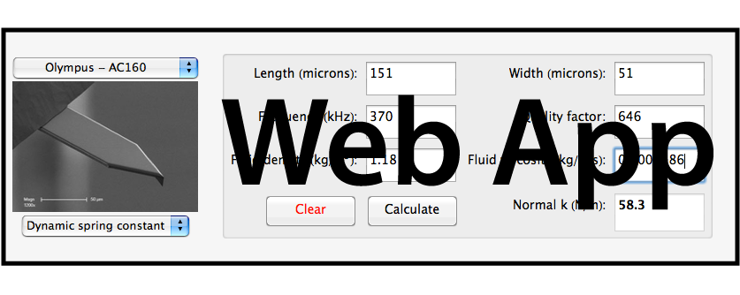
where L and b are the length and width of the cantilever, respectively, ρ is the density of the fluid, ωf and Qf are the (radial) resonant frequency and quality factor of the fundamental resonance peak, respectively, and Γif is the imaginary part of the hydrodynamic function given by Eq. (20) of Ref. [2]. In order to assist the reader, the Sader method has been implemented in an online calibrator, meaning that no code needs to be written by the user. Furthermore, the authors have made available Mathematica ® notebooks for download which perform the calculations. Torsional Sader method
Recently [4], the Sader method has been extended to allow
calibration of the torsional spring constant of rectangular AFM cantilevers,
using the result
where L and b are the length and width of the cantilever, respectively, ρ is the density of the fluid, ωt and Qt are the (radial) resonant frequency and quality factor of the fundamental torsional resonance peak, respectively, and Γit is the imaginary part of the hydrodynamic function given by Eq. (20) of Ref. [5]. Again, in order to assist the reader, the Torsional Sader method has been implemented in an online calibrator. Also, the authors have made available Mathematica ® notebooks for download which perform the calculations. General Method for Arbitrary Small Bodies
The extension of the Sader method to cantilevers of arbitrary shape was recently
presented [6], [7]. This includes an explanation of the underlying physical basis
of the method, its validity in the presence of nonidealities, such as added spheres
or tips, and its general applicability to small elastic bodies of arbitrary shape
and composition.
References
Home - Background theory - Online calibration - Mathematica files - Bibliography |